Whiskeytown Project

The key to cost-effective sediment reduction is prevention, not treatment of what has already happened. Therefore, erosion inventories must evaluate all existing and potential problems along roads and

document the amount of erosion that may potentially occur, particularly at road and
stream intersections (crossings). Professional training in geomorphology is essential for those involved in evaluating erosion activity. Without the prerequisite training, critical indicators of instability may be overlooked, yielding erroneous results and a potentially misguided watershed restoration program (Spreiter, 1992). It is recommended that the inventory team conduct a thorough study of all available air photos. Historic air photo analysis is a good way to determine even the obscured and overgrown roads, the history of road construction and the age of existing erosion features. The most important features to inventory are the intersections of all roads and streams, including sites where skid roads, trails, and transmission line easements cross headwater swales, gullies, and intermittent or perennial streams.

Why the Paige Bar Watershed?

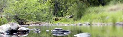
The 120 ha (300-ac) Paige-Bar subwatershed was chosen as the demonstration subwatershed for the pilot project. The sub-watershed is located in the lower Clear Creek watershed near the Whiskeytown National Environmental Education Development (N.E.E.D.) Camp. The demonstration sub-watershed was extensively logged and roaded in the 1960’s, and most recently in 1973, just prior to NPS acquisition of the lands. The “demo” watershed has within its boundaries approximately 2 kilometers of main use road (Peltier Valley Road) and several kilometers of old haul roads, including the badly eroded Logging Camp Road. These old roads are currently used for recreation, primarily hiking, mountain biking, and horseback riding. There are also old landings built in the stream channels that are actively eroding and chronically producing sediment.

The Inventory

Prior to field inventory work, the entire micro-drainage network of the Paige-Bar subwatershed was drawn onto the Igo quadrangle (7.5 minute) topographical map. The roads and streams were also delineated on mylar (clear) by laying the mylar over aerial photos and orthophotos. Recent as well as older stereo air photos were studied because problem areas that are still eroding but currently hidden by dense vegetative regrowth are often clearly visible in the photos taken immediately after disturbance. Historic air photo analysis is an efficient way to become thoroughly familiar with the drainage network, history of road construction, timber harvest, and other disturbances.

The inventory work was completed in the summer and fall of 1996. During this “ground truthing” phase the students worked in groups as an interdisciplinary team. It is important to get as many perspectives as possible while inventorying the landforms and asking “why is it like this?”. The geomorphic perspective is very important so the students were given some training in geology and fluvial processes. The class was taken on field tours of nearby Grass Valley Creek watershed to evaluate the efficacy of the treatments used there.

The restoration goals for Whiskeytown National Recreation Area include restoring naturally functioning ecosystems by treating and removing scars on the landscape, such as roads. Historic air photos reveal an extensive network of logging roads throughout the park. Many of the roads visible on the air photos were the long-abandoned haul roads, while miles of skid trails and small “one time use” access roads, called “ghost roads”, were invisible. Students performed field reconnaissance and developed road inventory methods combined with GIS technology to evaluate the potential for: 1) Road failures at stream crossings; 2) Road diversion gullies; and 3) Road-induced landslides

The class developed inventory forms based on advice from Redwood National Park’s Terry Spreiter and geologist Neal Youngblood. The strategy used divided the inventory into two distinct areas; the “site” which is where the road crossed a drainage, and the “road segment” which is the road length in-between sites. The road erosion inventory form therefore has two sections, one for sites (swale or stream crossings), and one section for road segments. As the teams proceeded down the road, the appropriate section - either site or segment - was filled out. Photographs were taken of each site or segment. Road condition, accessibility, width, and length were also noted and recorded on the data sheet.

Data was collected for the sites, including the type of site, i.e., stream crossing, headwater swale crossing, spring, crossroad drain, or other. The amount of fill in the site was estimated as an order of magnitude ranging from small (1-5 m³) to extra-large (greater than 50 m³). Potential for future erosion was evaluated and recommended treatment(s) were suggested. Possible treatments included a shallow dip (10% of the fill removed), culvert replacement, a large dip (50% of the fill removed), or complete crossing removal (100% of the roadfill would be excavated). Justifications for the treatment recommendations were also recorded. Data was also collected for the road segments. The amount of fill in the road wedge was estimated in cubic yards, and the potential for future erosion was assessed as high, moderate, or low. Based on this information, a potential treatment was recommended, i.e., outslope, outslope with rolling dip, or recontour (partial or complete road removal).

Estimates of potential erosion volume are by nature imprecise, inconsistent, and difficult because the numbers are calculated from estimates of dimensions of as yet unformed erosion features. Therefore, the dimensional numbers collected in the field are extremely subjective and should not be used as anything more than an indicator of the order of magnitude of what might occur in a major (50 year +) storm. The Watershed Restoration class looked at the disturbed lands, especially at the road and stream crossings (x-ings), and tried to determine the boundary between the fill and the undisturbed ground. The question asked was “Where was the road cut and where was it filled?”. The identification of fill versus native ground is not always obvious, thus the need for a strong geomorphic background. The amount of fill was put into relative categories, small (1-5 m³), medium (5-20 m³), large (20-50 m³), and extra-large (greater than 50 m³). The student teams used a unique technique to calibrate and visualize the amount of roadfill in channels. A “small” became a Volkswagon Bug, a van (the volume our college van would occupy) was a “medium”, a Greyhound Bus became synonymous with a “large” amount of fill, and finally an “extra-large was equated to the volume a triple-wide mobile home might occupy.

The information collected was entered into a database and then linked to a geographic information system (GIS). The Shasta College Engineering and GIS students got involved at this point and GIS maps were developed (Figure 6). The attributes for each site and segment can now be queried with Arcinfo™. Even the “before” photographs have been digitized and entered into the database. This should prove to be an invaluable monitoring tool.